Disclaimer: this is an article on cool and fun tools and best practice, tips to find you find a good job in Silicon Valley especially among the tech unicorns. This is a personal blog and I am not a career counselor. That being said, I have been to tons of company events and can give some good insights.
For recent graduates:
Utilize your college / University career center, website
Feeling stuck in your mid career? Need a renewal? Haven't worked for a while? Consider being a part-time student for a master degree, or an online degree, but look for jobs at the same time. Don't just get one degree after another. Trust me I know how nice that is. I did it. But it can also be a trap.
For new moms: some corporate responsibility programs offer career job positions who women who have left work for child rearing. For example, Lending Club's recent job post on LinkedIn (Feb 2019) "The Path Forward Return to Work program at LendignClub is a 16- week paid returnship for ... mother". Google "return to work", "returnship".
Tools for interview preps:
Pramp for technical interviews, data science and product management
Capstone Proposal
Technical proposal highlighing the real world problem, research done so far, and your research and approach in the field. Identify the correct datasets. Use Kaggle or DevPost to identify a problem. Proposal has to match final project. Kaggle might have already defined some of the requirements. Basic datasets like the MNIST cannot be used. Can use a representative sample of a large dataset. In essence Kaggle is the fastest. Discuss each section of the proposal. Be as detailed as possible. The requirement is high. As always Rubric is the most important evaluation criteria. Provide all important supplement materials.
Anaconda is a technical package manager that is especially useful for data scientists. It can save hours of configuration for windows users. It is a bit bulky but it is data scientists’ friend and must have toolkit in academia. Researchers use anaconda to manage their packages, instead of Python pip all the time.
Are you working on an Udacity nanodegree? Are you using Kaggle for data competitions? Are you doing graduate level research and studies? Anaconda may be your friend!
Staff writerSunsays she uses anaconda to install all packages on her windows gaming computer, so that she can easily use the GPU to train her neural networks. She’s a Mac user and want to spend minimal time configuring and setting up a development environment on windows. It just works. All her Jupyter Notebooks run, and it was easy to use CUDA to train her models on GPU.
Convention$prefix means it is a command line command which distinguishes from a python or Javascript line of code. Don’t copy and paste the dollar sign when using our cheatsheet.
Prefer a PDF version of the cheatsheet? Let us know in the comments or email us at hi@uniqtech.co
Installation and Uninstall
Miniconda is a lite version (light version) of anaconda. It takes less space but has the essentials of a data scientist toolset. Udacity sometimes suggests its students install miniconda.
Forcefully remove miniconda or anaconda. Use only if you know what you are doing.~/is the home path on Mac. You need to locate where your miniconda is installed on your computer first.
$ rm -r ~/miniconda
Anaconda offers an IDE called Spyder.It’s a desktop, visual GUI, which is easy to use and navigate. Pro tip: Usecommand+Mto open the matrix helper to quickly enter matrix data.
List all installed conda package
$ conda list
Install opencv with conda. This command does not work all the time. If fails, search stack overflow.
$ conda install -c conda-forge opencv
Using Anaconda
Anaconda Environments
List all environments.Forgot the name of the environment you created? Use this command to list all environments.
$ conda env list
Create an anaconda environment.create -ncreates a new environment. We also specified the version of python we want to usepython=3 . We also added the package we want to install as a suffix.
$ conda create -n my_env numpy
Activate an anaconda environment.How to activate Anaconda environment? Use the command below
$ conda activate my_env
Use Anaconda to Install Data Science Packages
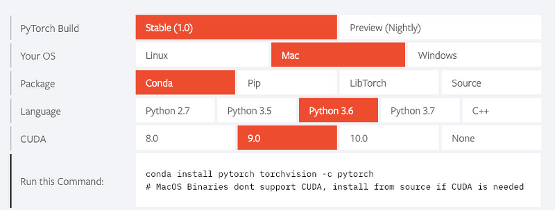
Use Anaconda to install Pytorch (check the Pytorch documentation for the latest and greatest). Only run this command after you finished the recommended anaconda initial install.
$ conda install pytorch torchvision -c pytorch
Install pytorch and torchvision using Anaconda on Mac and Windows
See the Pytorch documentation above. You can toggle and check how to instal using Pip as well if that’s easier.
Advanced Use of Anaconda
Using Anaconda in production | Using Anaconda for Reproducible Research
It may be apparent now that conda uses .yamlto manage configuration and requirement files similar to modern Ruby on Rails and Node.js, front end development best practice.
conda update jupyterUpdate the kernel to the latest version of Pythonconda install python=3Make Jupyter Notebook aware of new anaconda environmentipython kernel install --name my_env_name --user . So the kernel can be set.
Lesson
1 Part 10 (3.1.10) — training loop, batch calculation, trainloader
helps load data in batches, sometimes we add accumulative loss,
sometimes average loss (outside the training loop). Cross entropy loss
is a two step calculation, it takes in scores or logits, outputs
AVERAGED loss not full loss.
(3.1.11) Jupyter notebook for MLP
(3.1.12)
(3.1.13)
One Solution — Define MLP Layer. Because the model returns a vector of
scores, need to use max() to find the top score and then map it to the
top class. There’s a practical code snippet to calculate class accuracy
and distribution (if classes are evenly distributed) Best practice:
think about when to activate versus not. Training loss should decrease
over time. Use model.eval() during inference, and then switch it back to
model.train() for training. Lesson 5 Part 10 (3.5.10) — Cross Entropy Loss, Log Softmax, Log Loss NLLLoss() average loss over minibatch, training process
(3.1.14) — Model Evaluation: How
many epochs to train before model is overfitting? How do you know?
Split data into train test validation set!! It’s an important concept in
practice. Model only looks at training set during training and weight
updating. After each epoch, the model is evaluated against the validation set (note in most of deep learning this is referred to as testing set). The model never performs back propagation on the validation set. The validation set tells us if the model is generalizing well. Test set (note:
in most deep learning this is known as the validation set) is withheld
until the very end, after training, all together. It checks the accuracy
of the trained model. The withheld dataset is the best simulation we
have on hand of data that the model has never seen before.
(3.1.15)
Validation Loss: choose a percentage, do random subset sampling to get
the dataset partition. How to turn a dataset into indices, shuffled then
choose which index to get into subsets of validation dataset. Use
SubsetRandomSampler() (skip to the code snippet section to see the
documentation). Use validation set to figure out programmatically when
to stop training.
3.1.18 conceptually images are divided and consumed in regions by The
algorithm. If image is divided into quadrants, there are only 4 hidden
node onlyeach see a quarter of the image. Excellent visualization of how
CNN local connectivity sparsity works!! Very good Can have 2 or more
collections of hidden nodes, only seeing regions of an image. Red nodes
in the hidden layer only connected with red nodes in the image layer.
Finding patterns any way in an image — weight sharing.
3.1.19 Filter convolutional Can retain spatial info. Using a convolution layer, kernel or filter scans the original image for patterns, spans filter layers
3.1.20
Filters & Edges: introduction — shapes, pattern of intensity in an
image, distinguish object / figure and background detect changes in
intensity.
3.1.21
frequency in image: high frequency means more oscillation for the same
time interval, frequency can also be measured by amplitude and
oscillation. Rate of change is high for objects of relevance, but for
background it is low.
(3.2) Cloud Computing with AWS and get Udacity AWS credit (3.3) Transfer Learning (3.3.1) Intro to transfer learning using pre-trained CNN architecture such as VGG-16 model with 1000 class output, and ResNet (3.3.2)
Visualize VGG architecture (with feature extraction layers and linear
layers before output). Only need to train the final layers. Illustrate
where the transfer learning happens in the last couple of layers.
3.3.2
Useful layers: Convolutional Neural Network (CNN) hierarchical feature
extract architecture and removable classification layers for transfer
learning. Extract features and patterns. If available dataset is small,
but it’s similar to imagenet dataset, can use this architecture
pre-trained for our project.
3.3.3
A very very detailed section! Lots of content here. What to do when
dataset is large and different from ImageNet? Transfer learning with
Inception by Sebastian Thrun and Stanford University partners to
classify skin cancer, last densely connected layer was removed. Added a
new fully connected layer with an output size we define. Output layer
for each disease class. Random weight initialization was used for the
final layer. Intialized the rest of the weights using pre-trained
weights. Re-train the entire network in the end. What to do with the
four scenarios of new data:
New data set is small, new data is similar to original training data.
New data set is small, new data is different from original training data.
New data set is large, new data is similar to original training data.
New data set is large, new data is different from original training data.
3.3.4
VGG Model & Classifier: will train the last 3 fully connected
layers. Since the final layer is new added, with the number of classes
relevant to the new dataset, this process is called TRAIN. The 2nd and
3rd to last layer were there before, so it is called FINE TUNING when it
is trained again. Check if CUDA is available. Use Pytorch ImageFolder
class, which assumes the following conventions: the folder names are
correct label names, e.g. all sunflower images should be in the
sunflower folder. VGG model expects to see 224x224 images as input. use
transforms.RandomResizedCrop(224) to prep inputs. DataLoader class loads
data in BATCHES. How to access specific VGG16 layers and fully
connected layers. Print out in_features and out_features.
3.4.2
how to initialize constant weights and short fall of init constant
weights. def __init__(self, hidden_1, hidden_2, constant_weight=None): …
if constant_weight is not None: … #set constant_weight as an optional
parameter. nn.init.constant_(variable_to_set, value_to_set) e.g.
nn.init.constant_(m_bias, 0)
3.5.5
Defining & Training an autoencoder. One compresses one unzips. Init
a NN, with two fc’s one for encoding one for decoding. Dimensions
(input, encoding_dim) and (encoding_dim, input) so that it can be
connected and the result is comparable. Criterion compares input image
and output image. 3.5.6 test auto encoder by looking at its output
image. reshape images back to original MNIST style output =
output.view(batch_size, 1,28,28)
3.5.6
A simple solution: can observe where training loss decreases
drastically versus slowly. One way to check how the model is doing.
Compare original image to reconstructions. Can display it. Can flatten
image to autoencoder, reconstruct to 28x28 again. See when the training
loss is decreasing drastically vs not decreasing. Test autoencoder,
display an encoded image to see how ti turned out.
3.5.7
learnable upsampling; rather using a linear layer, can also use a
convolutional layer, which preserves spatial information. The encoder
now becomes a hierarchical structure with some CNN layers, that
typically downsample (such as max pooling). How to go from compressed to
reconstructed? Want to reverse the down sampling, upsampling (unpool).
Such as using an interpolation technique nearest neighbors. This is just
copying the existing values. But can train and learn how to upsample an
image effectively. Tranpose convolutional layer. Dubbed
de-convolutional layers with learnable parameters. It’s not undoing CNN.
3.5.7
Learnable upsampling: to reverse the encoding process, want to decode,
increase image dimensions. Reverse the encoding pooling by unpooling.
Interpolate results from existing pixels. Nearest neighbor, use the
existing value as value for all its neighbors, effectively copying the
number. There are advanced ways to upsample. Example, tranpose
convolutional layer, has learnable parameters, de-convolutional layers,
upsample existing values using filter wegiths. 3.5.8 Review
convolutional process. Math behind Tranpose Convolutional Layer. Useful
important visualization of strides. Strides of 2 means, it will move to
the right by 2 pixels at a time also move down 2 pixels at a time.
Stride value is roughly input to output dimensions! Very important.
The review material is too detailed to fit into a single blog post. I broke it down to 10 parts. See each link below. It's a detailed outline, review, and notes on each section of the MLND by Udacity.
Lesson
1 Part 10 (3.1.10) — training loop, batch calculation, trainloader
helps load data in batches, sometimes we add accumulative loss,
sometimes average loss (outside the training loop). Cross entropy loss
is a two step calculation, it takes in scores or logits, outputs
AVERAGED loss not full loss.
(3.1.11) Jupyter notebook for MLP
(3.1.12)
(3.1.13)
One Solution — Define MLP Layer. Because the model returns a vector of
scores, need to use max() to find the top score and then map it to the
top class. There’s a practical code snippet to calculate class accuracy
and distribution (if classes are evenly distributed) Best practice:
think about when to activate versus not. Training loss should decrease
over time. Use model.eval() during inference, and then switch it back to
model.train() for training. Lesson 5 Part 10 (3.5.10) — Cross Entropy Loss, Log Softmax, Log Loss NLLLoss() average loss over minibatch, training process
(3.1.14) — Model Evaluation: How
many epochs to train before model is overfitting? How do you know?
Split data into train test validation set!! It’s an important concept in
practice. Model only looks at training set during training and weight
updating. After each epoch, the model is evaluated against the validation set (note in most of deep learning this is referred to as testing set). The model never performs back propagation on the validation set. The validation set tells us if the model is generalizing well. Test set (note:
in most deep learning this is known as the validation set) is withheld
until the very end, after training, all together. It checks the accuracy
of the trained model. The withheld dataset is the best simulation we
have on hand of data that the model has never seen before.
(3.1.15)
Validation Loss: choose a percentage, do random subset sampling to get
the dataset partition. How to turn a dataset into indices, shuffled then
choose which index to get into subsets of validation dataset. Use
SubsetRandomSampler() (skip to the code snippet section to see the
documentation). Use validation set to figure out programmatically when
to stop training.
(3.2) Cloud Computing with AWS and get Udacity AWS credit (3.3) Transfer Learning (3.3.1) Intro to transfer learning using pre-trained CNN architecture such as VGG-16 model with 1000 class output, and ResNet (3.3.2)
Visualize VGG architecture (with feature extraction layers and linear
layers before output). Only need to train the final layers. Illustrate
where the transfer learning happens in the last couple of layers.
3.3.2
Useful layers: Convolutional Neural Network (CNN) hierarchical feature
extract architecture and removable classification layers for transfer
learning. Extract features and patterns. If available dataset is small,
but it’s similar to imagenet dataset, can use this architecture
pre-trained for our project.
3.3.3
A very very detailed section! Lots of content here. What to do when
dataset is large and different from ImageNet? Transfer learning with
Inception by Sebastian Thrun and Stanford University partners to
classify skin cancer, last densely connected layer was removed. Added a
new fully connected layer with an output size we define. Output layer
for each disease class. Random weight initialization was used for the
final layer. Intialized the rest of the weights using pre-trained
weights. Re-train the entire network in the end. What to do with the
four scenarios of new data:
New data set is small, new data is similar to original training data.
New data set is small, new data is different from original training data.
New data set is large, new data is similar to original training data.
New data set is large, new data is different from original training data.
3.3.4
VGG Model & Classifier: will train the last 3 fully connected
layers. Since the final layer is new added, with the number of classes
relevant to the new dataset, this process is called TRAIN. The 2nd and
3rd to last layer were there before, so it is called FINE TUNING when it
is trained again. Check if CUDA is available. Use Pytorch ImageFolder
class, which assumes the following conventions: the folder names are
correct label names, e.g. all sunflower images should be in the
sunflower folder. VGG model expects to see 224x224 images as input. use
transforms.RandomResizedCrop(224) to prep inputs. DataLoader class loads
data in BATCHES. How to access specific VGG16 layers and fully
connected layers. Print out in_features and out_features.
3.4.2
how to initialize constant weights and short fall of init constant
weights. def __init__(self, hidden_1, hidden_2, constant_weight=None): …
if constant_weight is not None: … #set constant_weight as an optional
parameter. nn.init.constant_(variable_to_set, value_to_set) e.g.
nn.init.constant_(m_bias, 0)
3.5.5
Defining & Training an autoencoder. One compresses one unzips. Init
a NN, with two fc’s one for encoding one for decoding. Dimensions
(input, encoding_dim) and (encoding_dim, input) so that it can be
connected and the result is comparable. Criterion compares input image
and output image. 3.5.6 test auto encoder by looking at its output
image. reshape images back to original MNIST style output =
output.view(batch_size, 1,28,28)
3.5.6
A simple solution: can observe where training loss decreases
drastically versus slowly. One way to check how the model is doing.
Compare original image to reconstructions. Can display it. Can flatten
image to autoencoder, reconstruct to 28x28 again.
3.5.7
learnable upsampling; rather using a linear layer, can also use a
convolutional layer, which preserves spatial information. The encoder
now becomes a hierarchical structure with some CNN layers, that
typically downsample (such as max pooling). How to go from compressed to
reconstructed? Want to reverse the down sampling, upsampling (unpool).
Such as using an interpolation technique nearest neighbors. This is just
copying the existing values. But can train and learn how to upsample an
image effectively. Tranpose convolutional layer. Dubbed
de-convolutional layers with learnable parameters. It’s not undoing CNN.
3.5.8 Tranpose Convolution: Math behind Tranpose Convolutional Layer